Spotxel® Reader: Plate Reader & Microarray Image Analysis
Spotxel Reader® turns smartphones into a handy and quality microplate reader. The free app enables reading and analysis of multiple samples in parallel in plate formats:
- Capturing: Take picture of the microplate.
- Reading: Detect and measure color signal in the microplate wells.
- Analysis: Annotate the microplate, specify the assay’s standards concentration, and derive the unknowns’ concentration.
The app also supports image analysis of assays with samples in row, column, or microarray formats.
To start with, install the app from the app store with the following links, and explore its functionality with this sample image and its setting in Figure 7 if you do not have one.
|
|
|
Camera calibration and image capture
The Camera page (Figure 1) provides a virtual plate which highlights the wells at the plate’s center and corner. You can adjust the size and the distortion factor of this virtual plate to tune for the best position and angle of the camera to the real plate.
The calibration parameters are saved upon the image capturing, thus it might need to be calibrated only once. This is particularly useful if a fixed holder (Figure 1) is employed. In addition, careful calibration aligns the captured image with the real plate, enabling image analysis without further alignment.
 |
Image analysis
The Image Analysis page (Figure 2) supports detection and quantification of the wells’ color signal. You can choose to analyze an image captured by the app or an available image on your phone (for iOS devices: from the Photo Library).
 |
Challenges to be addressed
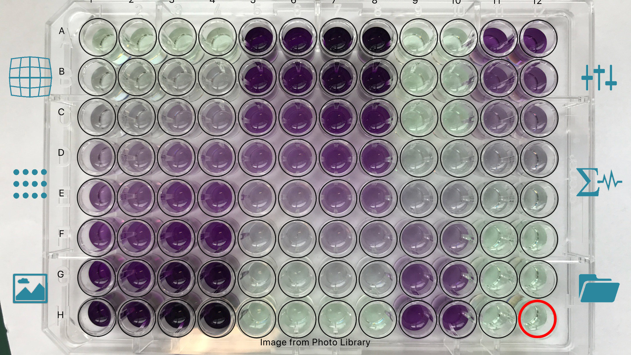
Consider the microplate image in Figure 3. Unexpected artifacts should be detected and processed. These include:
(1) Camera lens’ distortion effect and different view angles to the wells: The camera focuses at the plate’s center. Observe that the well signal at the plate center such as D6 or E7 is round, while those at the border such as A12 or G1 are elliptic.
(2) “Smearing” signal from neighbor wells: Consider well F3; the signal at its left side is due to well F2, while that at its bottom side is due to well G3.
 |
Signal Detection and Quantification
You can start processing the image after aligning the virtual microplate with the image. The detection and quantification of the wells’ signal takes a few seconds to some minutes, depending on the smartphone processor and the image resolution. The grid is then hidden for viewing convenience. The detected signal in each well is marked with a red boundary (Figure 4).
 |
Signal Detection Results
Observe the detected signal in Figure 4 and a close-up of the plate bottom-left corner in Figure 5. The signal detection procedure, whose result is illustrated by red boundary, is able to:
- Identify the significant region of the wells’ signal, regardless of their shape and color intensity.
- Exclude the “smearing” signal of the neighbor wells.
 |
Signal Quantification Results
The color intensity values are graphically reported in the virtual microplate in the Assay page (Figure 6), as well as in the classical table format in the Quantified Data page (Figure 10).
 |
Assay setup and colorimetric data analysis
By means of a virtual plate in the Assay page (Figure 6), we can define the wells’ name and notes and set the standards’ concentration. After signal quantification, this page depicts the wells in the color similar to that of the wells’ sample. Annotation is easy; simply select a well and type in the name or using the slider to set the concentration value.
 |
Having the wells’ color intensity and the standards’ concentration available, we can start the analysis to find the unknowns’ concentration value. The Standard Curve page (Figure 8) depicts a chart with the standard curve as the green curve and the standards’ coordinate as blue dots.
 |
The unknowns’ concentration values are derived from the standard curve. They are reported directly in the Assay page (Figure 9), as well as in the table in the Quantified Data page (Figure 10).
 |
Table of Quantified Data
The Quantified Data page presents a table containing both the annotation and the quantified data of the microplate. These include the wells’ address, name, notes, and their color intensity and concentration value if available. The table data can be exported to a CSV file for report o further analysis.
 |
Quality
The analysis results exhibit very good correlation (Figure 11) with those of a popular plate reader.
 |
Product Updates
12 Dec 2018 - Demo video of trajectory and 3D-reconstruction on autonomous vehicle dataset.
09 Oct 2018 - Demo video of object detection and multi-object tracking on autonomous vehicle...
30 Aug 2018 - Demo video for multi-object tracking on self-driving data is available at YouTube.